Python matplotlib : colormaps (colormap 종류, cmap)

 

 

 

matplotlib에서는 색상의 그라데이션을 사용할 때가 있습니다.

주로 어떤 데이터셋에서 숫자가 낮을 수록 흰색, 숫자가 높을 수록 검은색 이런 식으로 색상의 그라데이션을 통해 숫자의 크기를 나타낼 때가 있는데 이런 경우에 그라데이션을 자주 사용하죠.

 

matplotlib에는 이미 내장된 다양한 종류의 그라데이션 세트가 있으며 이를 colormap이라고 합니다.

 

colormap의 종류는 matplotlib.colormaps를 통해서 알 수 있습니다.

 

from matplotlib import colormaps

print(colormaps)


-- Result
'magma', 'inferno', 'plasma', 'viridis', 'cividis', 'twilight', 'twilight_shifted', 'turbo', 'Blues', 'BrBG', 'BuGn', 'BuPu', 'CMRmap', 'GnBu', 'Greens', 'Greys', 'OrRd', 'Oranges', 'PRGn', 'PiYG', 'PuBu', 'PuBuGn', 'PuOr', 'PuRd', 'Purples', 'RdBu', 'RdGy', 'RdPu', 'RdYlBu', 'RdYlGn', 'Reds', 'Spectral', 'Wistia', 'YlGn', 'YlGnBu', 'YlOrBr', 'YlOrRd', 'afmhot', 'autumn', 'binary', 'bone', 'brg', 'bwr', 'cool', 'coolwarm', 'copper', 'cubehelix', 'flag', 'gist_earth', 'gist_gray', 'gist_heat', 'gist_ncar', 'gist_rainbow', 'gist_stern', 'gist_yarg', 'gnuplot', 'gnuplot2', 'gray', 'hot', 'hsv', 'jet', 'nipy_spectral', 'ocean', 'pink', 'prism', 'rainbow', 'seismic', 'spring', 'summer', 'terrain', 'winter', 'Accent', 'Dark2', 'Paired', 'Pastel1', 'Pastel2', 'Set1', 'Set2', 'Set3', 'tab10', 'tab20', 'tab20b', 'tab20c', 'grey', 'gist_grey', 'gist_yerg', 'Grays', 'magma_r', 'inferno_r', 'plasma_r', 'viridis_r', 'cividis_r', 'twilight_r', 'twilight_shifted_r', 'turbo_r', 'Blues_r', 'BrBG_r', 'BuGn_r', 'BuPu_r', 'CMRmap_r', 'GnBu_r', 'Greens_r', 'Greys_r', 'OrRd_r', 'Oranges_r', 'PRGn_r', 'PiYG_r', 'PuBu_r', 'PuBuGn_r', 'PuOr_r', 'PuRd_r', 'Purples_r', 'RdBu_r', 'RdGy_r', 'RdPu_r', 'RdYlBu_r', 'RdYlGn_r', 'Reds_r', 'Spectral_r', 'Wistia_r', 'YlGn_r', 'YlGnBu_r', 'YlOrBr_r', 'YlOrRd_r', 'afmhot_r', 'autumn_r', 'binary_r', 'bone_r', 'brg_r', 'bwr_r', 'cool_r', 'coolwarm_r', 'copper_r', 'cubehelix_r', 'flag_r', 'gist_earth_r', 'gist_gray_r', 'gist_heat_r', 'gist_ncar_r', 'gist_rainbow_r', 'gist_stern_r', 'gist_yarg_r', 'gnuplot_r', 'gnuplot2_r', 'gray_r', 'hot_r', 'hsv_r', 'jet_r', 'nipy_spectral_r', 'ocean_r', 'pink_r', 'prism_r', 'rainbow_r', 'seismic_r', 'spring_r', 'summer_r', 'terrain_r', 'winter_r', 'Accent_r', 'Dark2_r', 'Paired_r', 'Pastel1_r', 'Pastel2_r', 'Set1_r', 'Set2_r', 'Set3_r', 'tab10_r', 'tab20_r', 'tab20b_r', 'tab20c_r'

 

 

 

 

 

아래 코드는 colormap의 종류를 나타내어주는 코드입니다.

 

import matplotlib.pyplot as plt
from matplotlib import colormaps
import numpy as np


arr_values = np.linspace(0, 100, 10000)
max_row = 17

plt.figure(figsize=(10, 5))
fig, graph = plt.subplots(nrows=max_row, ncols=1)

for idx, cmap in enumerate(colormaps):
    graph_idx = idx % max_row
    print(idx, cmap, graph_idx)

    graph[graph_idx].pcolormesh([arr_values], cmap=cmap)
    graph[graph_idx].set_axis_off()
    graph[graph_idx].set_xlim(0, 10000)
    graph[graph_idx].text(x=10100, y=0,
                          s=cmap,
                          fontsize=10,
                          horizontalalignment='left',
                          verticalalignment='bottom')

    if idx != 0 and idx % max_row == 16:
        plt.savefig('cmap_{idx}.png'.format(idx=idx),
                    facecolor='#ffffff',
                    edgecolor='white',
                    format='png', dpi=300,
                    bbox_inches='tight',
                    pad_inches=0.025)
        plt.close()

        plt.figure(figsize=(10, 5))
        fig, graph = plt.subplots(nrows=max_row, ncols=1)

 

 

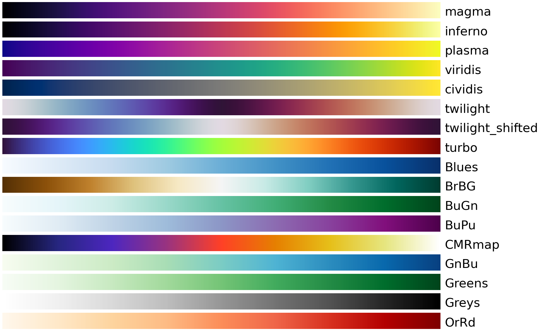
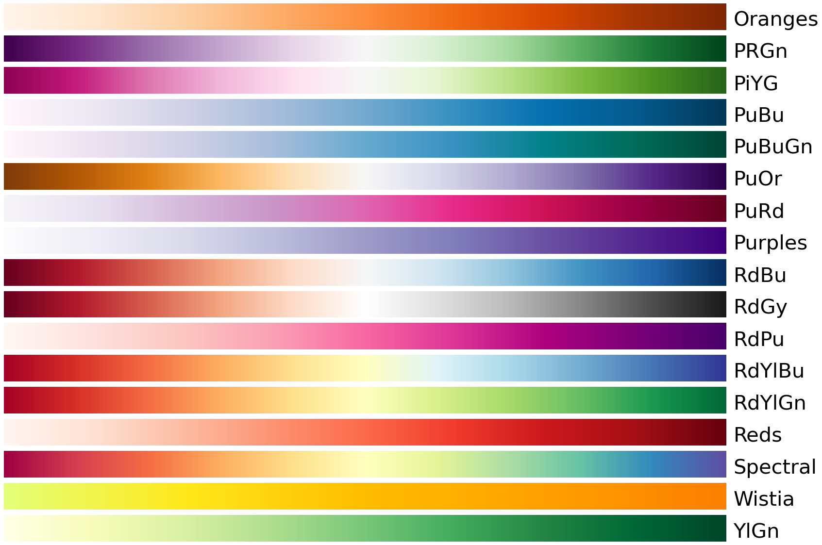
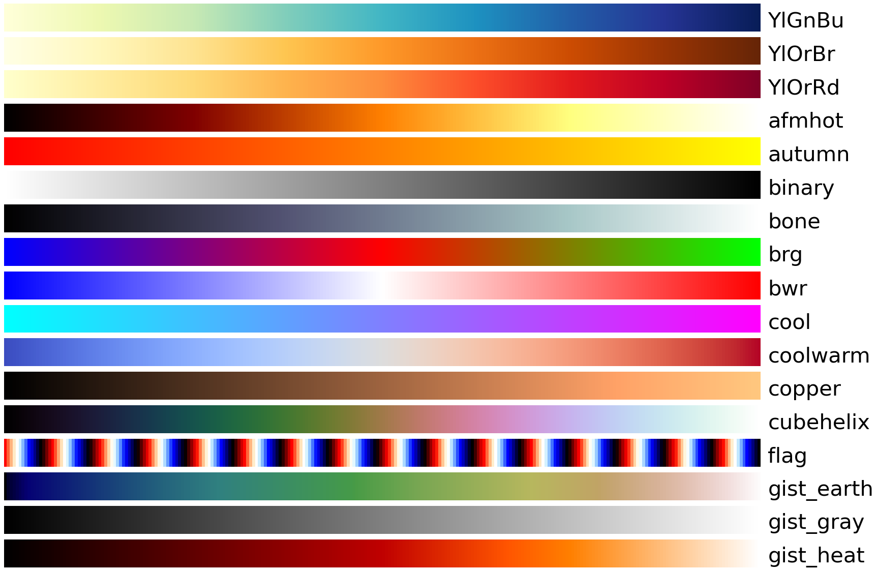
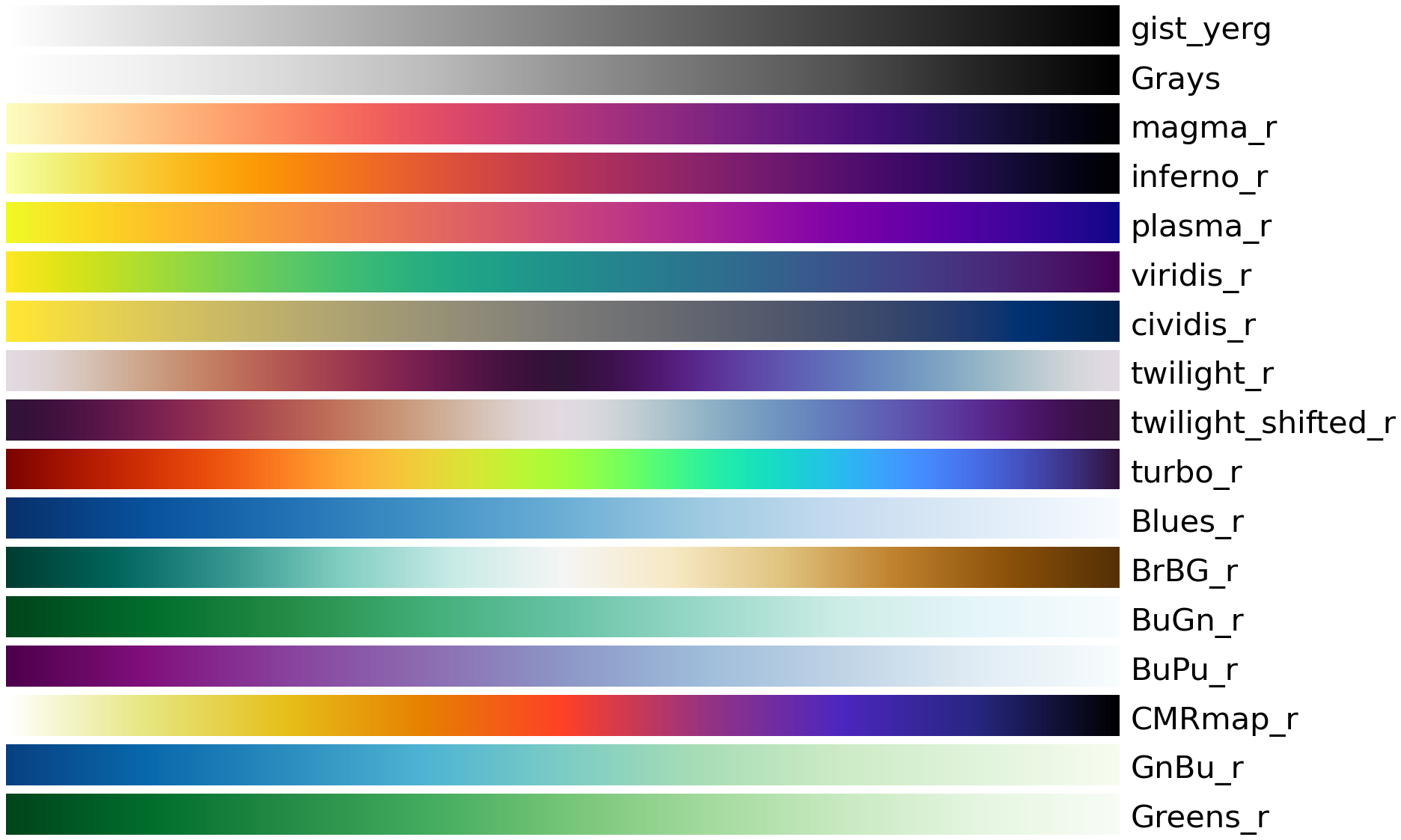
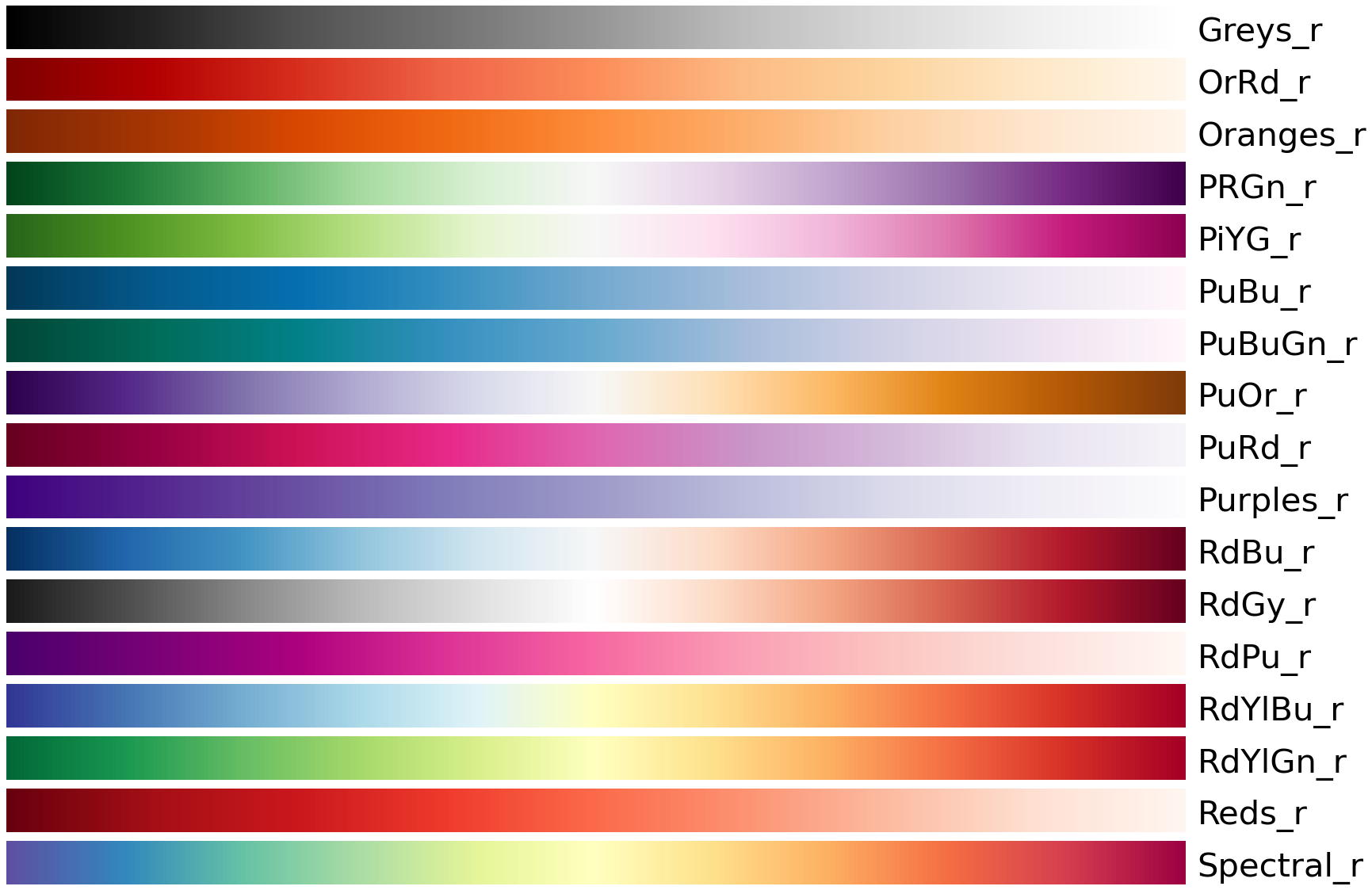
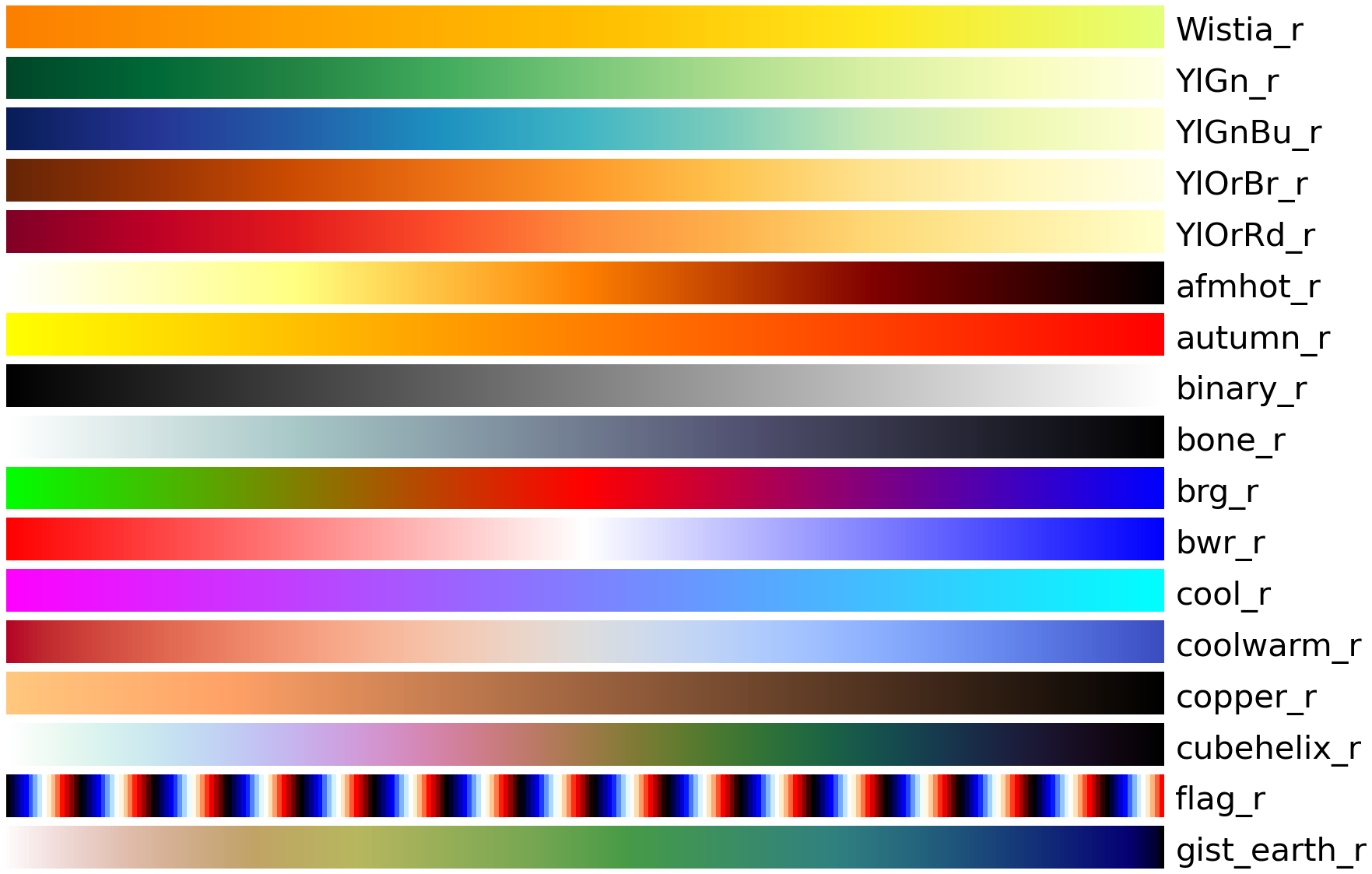
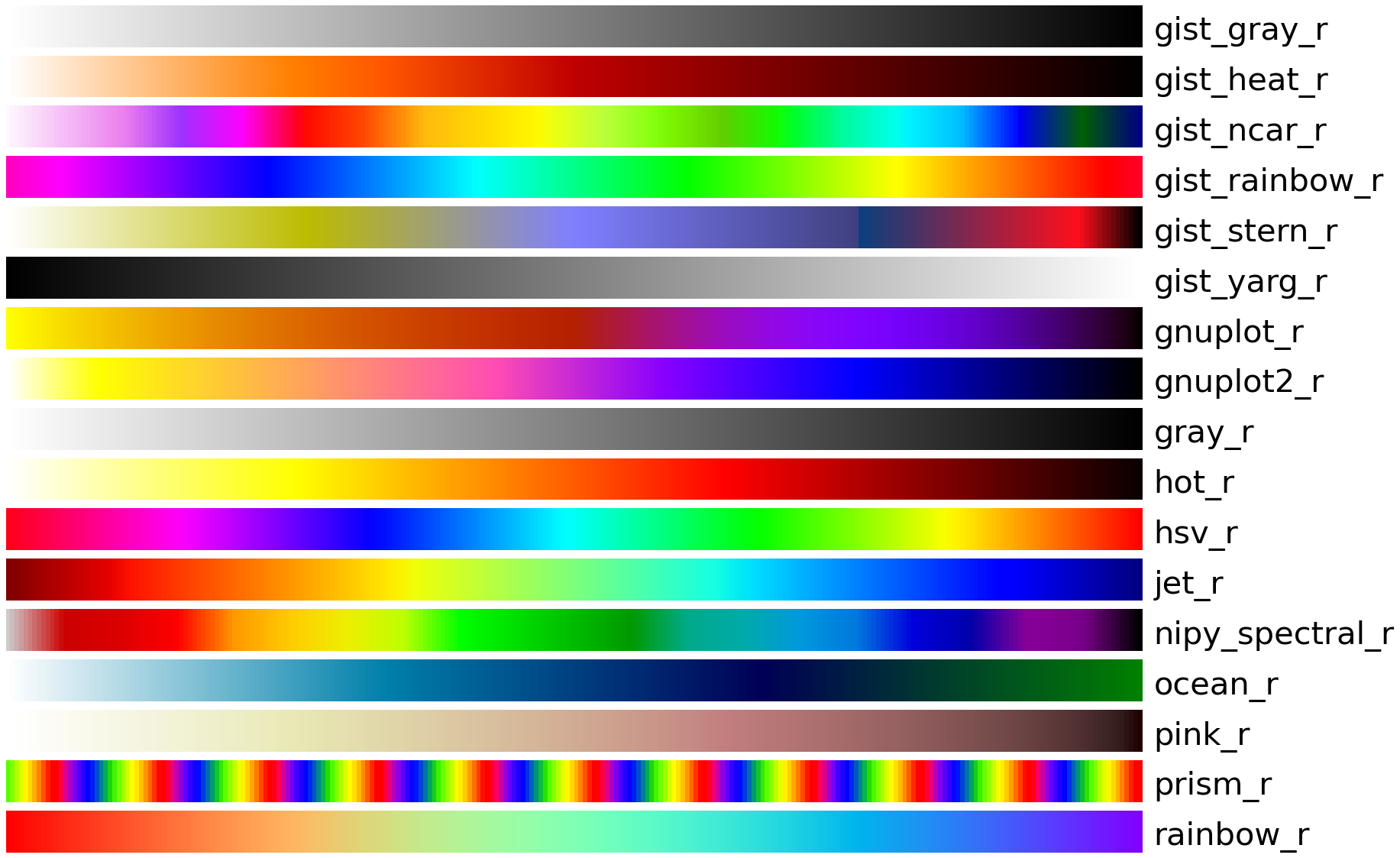
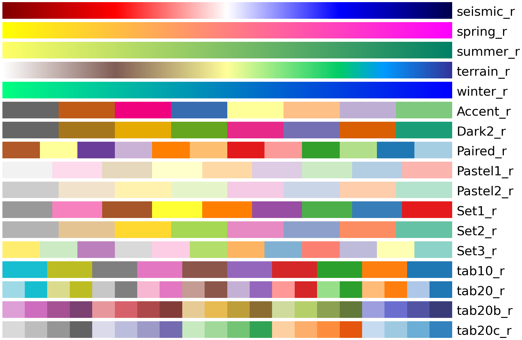
아래 이미지가 위 코드의 결과이며 색상을 보고 원하는 colormap을 선택해서 사용할 수 있습니다.

(matplotlib 버전에 따라 colormap의 종류는 좀 달라질 수 있습니다.)